In this article, we go further to discuss Markov chain Monte Carlo (MCMC) in the context of sampling methods, and how to design a MCMC algorithm for a specific sampling problem.
3. Sampling Methods in General
3.1. Motivations
Sampling methods (or simply "taking samples from a random distribution") has a braod range of applications:
- Estimate expectations and other statistics;
- Visualize a random distribution (as a histogram);
- Calculate area or integration (as a fraction of the bounding rectangular "box");
- Compute the normalizing constant to convert any functions to a probability distribution.
In addition, sampling method is relatively easy to implement. We will talk about some well-known methods in the following sections.
3.2. Monte Carlo method
The idea is simple, we first generate samples according to the distribution and then use sample mean as an approximation to the expected value.
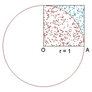
In the famous example of estimating the numerical value of $\pi$, we generate random samples within the uniform rectangle, and if we look at the quarter circle as a probability density function $f(x)$, the fraction of the area under that curve gives the probability of a random point falls within the circle. Mathematically, the idea can be expressed as the following: $$ P(\textrm{any point falling within the circle}) \\ = \frac{\int_{0}^{1}f(x)dx}{1} \\ = \frac{S_{1/4 \textrm{circle}}}{S_{\textrm{bounding rec.}}} = \pi $$
3.3. Importantce sampling
Strictly speaking, this is not a "sampling" method as it does not generate samples directly; instead, it is able to estimate expectation of a function over any distribution.
4. Markov Chain Monte Carlo
In this section, we will move one step forward, from theory to algorithms and see how a popular algorithm called Markov Chain Monte Carlo (MCMC) could help us solve various problems.
In Monte Carlo method, an underlying assumption is that all the sample points are independent and identically distributed (iid). Sometimes, this is not an efficient way of simulating a distribution (we will explain why in section 4.2). Unlike Monte Carlo method, MCMC takes samples from a Markov chain. Every new sample is conditioned on the previous sample according to some transition probability. It can be more efficient if the transition rule is well-desiged such that it somehow "guides" the samples afterwards to the regions where the probability density is high.
The theory about Markov chain has been covered in section 2. Here, we will focus on the algorithms which are used to generate markov chains for a target stationary distribution.
4.1. Why MCMC?
with the various sampling methods available as mentioned in the previous section, you might ask, "why do we need MCMC as another sampling technique?" To answer this question, let's introduce a simple example and see how we would simulate it without MCMC.
Example. Los Angeles' weather
If we assume there are only two types of weather: sunny and not-sunny, we can model the weather at different time as a Markov chain (state s1 is 'sunny' and s2 'not sunny'). The code below simulates the markov process using a pre-specified transition matrix P.
# In Los Angeles, as sunshine is much more common than other weathers, the
# transition matrix is assumed to be the following
# (from 'not-sunny' to 'sunny' is P12=0.5, from 'sunny' to 'not-sunny' is P21=0.1):
P = [[0.5, 0.5],
     [0.1, 0.9]]

# An initial distribution:
u0 = [0.5, 0.5]

N = 10 # The number of steps to simulate

from bisect import bisect
from random import random

def init_chain_state(u0):
  """
  u0: a list.
    The distribution of initial state.

  NOTE: Simulate the random state the same way as 'move_one_step()'; bisect
  is used to find the index efficiently。
  """
  target = [sum(u0[:i+1]) for i, ele in enumerate(u0)]
  x = random()
  state_index = bisect(target, x)
  # print(x, target, state_index)

  return state_index

# For testing purpose:
# u0 = [0.2, 0.5, 0.3]
# init_chain_state(u0)

def move_one_step(P, s_t, x):
  """
  In a Markov chain process, move from step t to t+1 according to the transition
  matrix.

  P: a list of list.
    The transition matrix.
  s_t: integer.
    The state at step t.
    1 for 'not-sunny', 2 for 'sunny'.
  x: float, between 0 and 1.

  # The code can be simplified, but we write out the "raw" idea here to
  # make it easy to compare to the algorithm description side by side.
  """
  if s_t == 1:
    # The if-statement below is the "naive" algorithm to select s_{t+1}:
    if x < P[0][0]:
      return 1
    elif x < P[0][0] + P[0][1]:
      return 2

  if s_t == 2:
    if x < P[1][0]:
      return 1
    elif x < P[1][0] + P[1][1]:
      return 2


def simulate_N_steps(P, u0, N):
  # Initial state:
  s_t = 1 if init_chain_state(u0)==0 else 2

  s_seq = []
  for i in range(N):
    x = random()
    s_t = move_one_step(P, s_t, x)
    s_seq.append(s_t)

  return s_seq

N = 1000
s_seq = simulate_N_steps(P, u0, N)
print(s_seq[-10:])
The process can be summarized as a "naive" solution to sample from a random distribution. Given a Markov chain with state space $S=\{s_1, s_2, ..., s_k\}$, we assume at step $n$, the state is $s_i$ ($X_n=s_i$). Then $X_{n+1}$ is determined from $s_i$ and a generated random number $x (x\in[0,1])$ in following way:
$\phi(s_i, x) = \left\{ \begin{array}{ll} s_1, x\in[0, P_{i,1}) \\ s_2, x\in[P_{i,1}, P_{i,1}+P_{i,2})\\ ...\\ s_k, x\in[\sum_{j=1}^{k-1} P_{i,j}, 1] \end{array} \right. $
Basically, there are two steps: First generate a random number $x$ second, find the next state corresponding to $x$. Notice that if $P_{i,j}$ is arbitrary for different $j$, then we have to determine the next state ($j\in[1,2,...,k]$) by finding where $x$ should be inserted into the cummulative probability (essentially a sorted list). Although we can use binary search to speed up the algorithm, it is still expensive if the state space is large.
In some cases, a Markov chain could have a high-dimensional state space and the size of the state space could be too large to handle in this "naive" method. That is when MCMC comes to rescue. Let's move on!
4.2. Metropolis algorithm
Let ${X_0, X_1, ..., X_n,...}$ be a Markov chain on a finite state space $E$. The Metropolis algorithm goes from the first sample $X_0$ like this:
Step 0:
- Initialize $X_0$;
Step $n$ to step $n+1$:
- Choose $y\in E$ with a stochastic selection matrix $Q(X_n, y)$;
- Choose $U$ at random uniformly in [0, 1]:
- Let $R(x,y), R\in [0,1]$ be a selection criteria. If $U < R(x,y)$ then accept the selection $X_{n+1}=y$;
- Otherwise, refuse the selection and set $X_{n+1}=X_{n}$.
If we think of a Markov chain as a random "jump" from one state to another every step, the Metropolis algorithm decomposes this random jump into two steps: First "propose" a candidate randomly according to $Q(x,y)$, then determine if we "accept" this proposed sample according to a probability function $R(x,y)$. Mathematically, the transition matrix is $$P(x_i, x_j)=P(X_{n+1}=x_j|X_{n}=x_i)=P(x_j|x_i)P(\textrm{accept}\ x_j | (x_i, x_j))$$ where the first term is modeled by $Q(x,y)$, and the second term is modeled by $R(x,y)$.
4.3. Does the Markov chain converges to the distribution you want?
Wait! But how do we know if the stationary distribution of this Markov chain is exactly the one we want to simulate (or draw samples from)? Very good question!
Suppose we are given a new algorithm (in the form of Metropolis algorithm), we have two routes to verify whether the Markov chain converges to the target distribution $\pi$.
Route 1. Starting from the transition matrix $P$ of the MC.
If we can show that P is irreducible and aperiodic, then we can try to verify whether $\pi P = P \pi$ holds. If it holds, congratulations, the M.C. will converge to $\pi$!
Route 2. Starting from the "selection matrix" $Q$ and the "accept matrix" $R$.
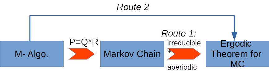
If we design $Q$ and $R$ using a special "receipy" as below, (we can show) the transition matrix always converge to $\pi$:
- $Q(x,y)>0\implies Q(y,x)>0$
- $h$ is a function mapping $(0, \infty)$ onto $(0, 1]$ s.t.: $h(u)=uh(1/u)$. The examples can be $h(u)=\frac{u}{1+u}$ or $h(u)=min(u,1)$
- Define $R(x,y)$ as:
$$R(x, y) = \left{
$$\begin{array}{ll} h(\frac{\pi(y) Q(y,x)}{\pi(x) Q(x,y)}), Q(x,y) \neq 0 \\ 0, Q(x,y)=0 \end{array} \right.
The resultant transition matrix is: $$P(x, y) = \left\{ \begin{array}{ll} Q(x,y)R(x,y), x\neq y\\ 1 - \sum_{x\neq y}P(x,y), x=y \end{array} \right. $$
SUMMARY
In this article, we introduced a powerful method Markov chain Monte Carlo. With other general sampling methods in mind, you will more appreciate how MCMC is useful for distributions with very large state space.
Metropolis algorithm is a popupar algorithm for MCMC. We not only talked about how to do it, but also explained why it converges to the distribution we want. Equipped with those powerful ideas, we are ready to make some experiments with them!
References:
[1] Olle Haggstrom, "Finite Markov Chains and Algorithmic Applications", Cambridge University Press 2002.
[2] Book section "Generating Samples from Probability Distributions": https://web.mit.edu/urban_or_book/www/book/chapter7/7.1.3.html
[3] Notes "Intro to Sampling Methods" (from PSU course "Math Tools for Computer Visions"): http://www.cse.psu.edu/~rtc12/CSE586/lectures/cse586samplingPreMCMC.pdf
[4] Videos about sampling methods (Machine Learning section 16 & 17), by "mathematicalmonk": https://www.youtube.com/watch?v=3Mw6ivkDVZc&list=PLD0F06AA0D2E8FFBA&index=132